Diagnostic Psychometrics

Introductions

W. Jake Thompson

• Ph.D. from KU’s REMS program
• Assistant Director of Psychometrics for Accessible Teaching, Learning, and Assessment Systems
• Research: Applications of diagnostic psychometric models,
  • Lead psychometrician and Co-PI for the Dynamic Learnings Maps assessments
  • PI for an IES-funded project to develo software for diagnostic models

Conceptual foundations

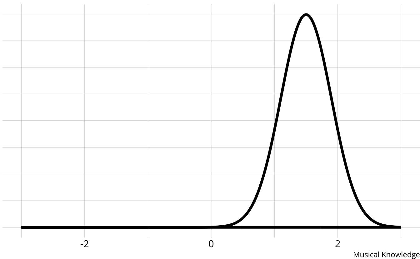
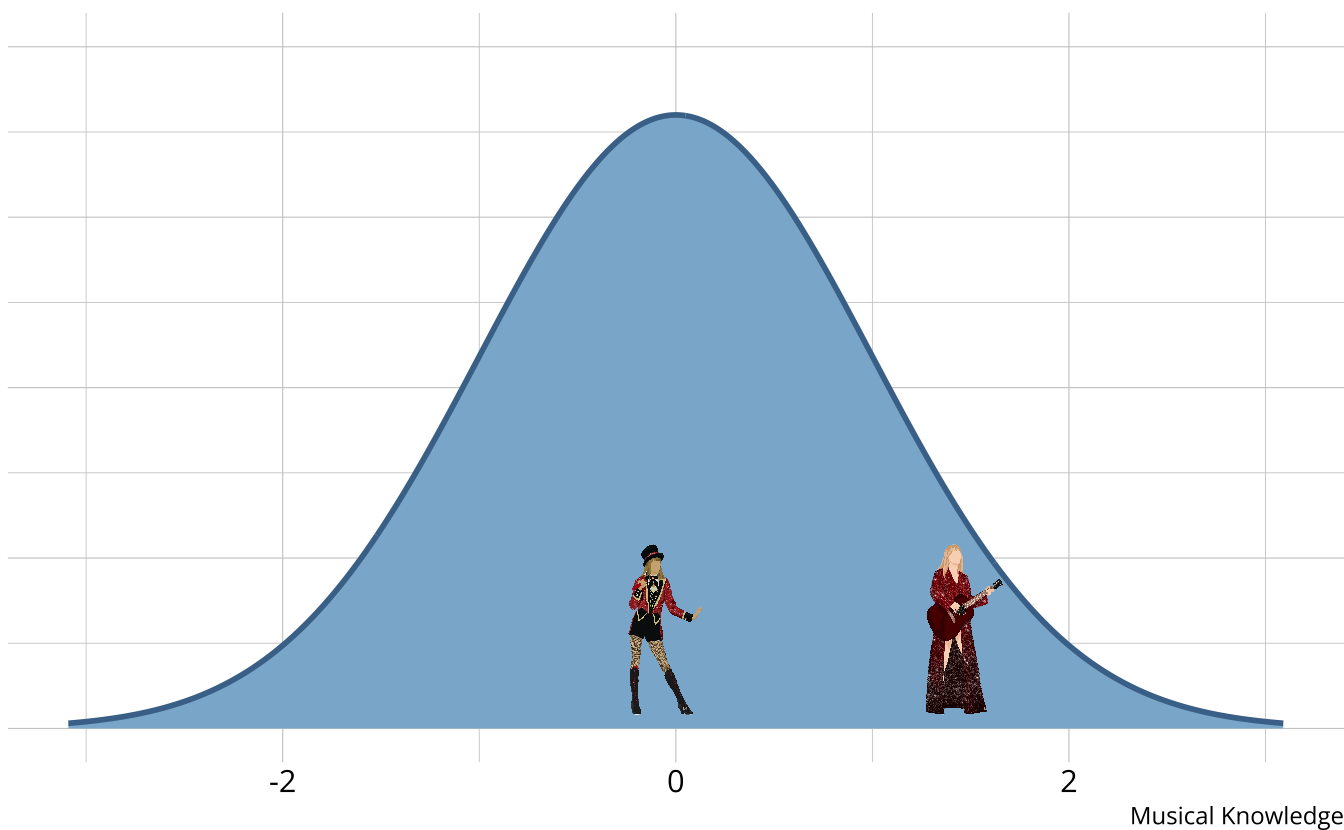
• Traditional assessments and psychometric models measure an overall skill or ability
• Assume a continuous latent trait

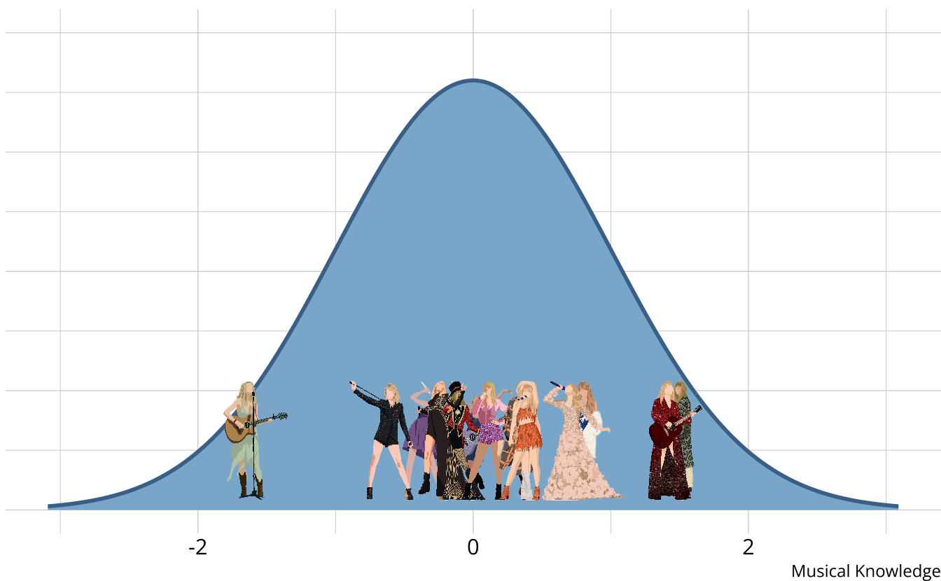
Traditional methods

• The output is a weak ordering of teams due to error in estimates
  • Confident Red (Taylor’s Version) is the best
  • Not confident which is second best (Speak Now (Taylor’s Version), folklore, Lover)
• Limited in the types of questions that can be answered.
  • Why is Taylor Swift (debut) so low?
  • What aspects do each album demonstrate mastery or competency of?
  • How much skill is “enough” to be competent?

Music example

• Rather than measuring overall musical knowledge, we can break music down into set of skills or attributes
  • Songwriting
  • Production
  • Vocals
  • Cohesion

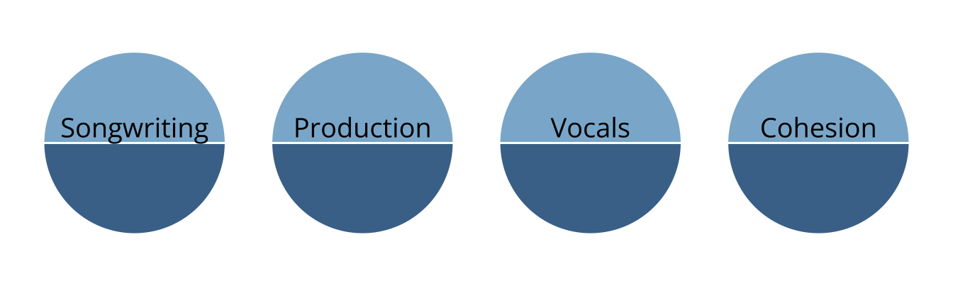
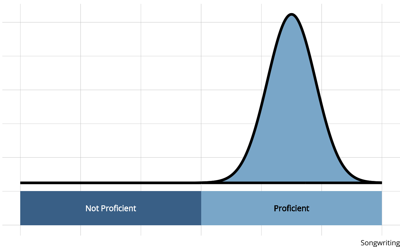
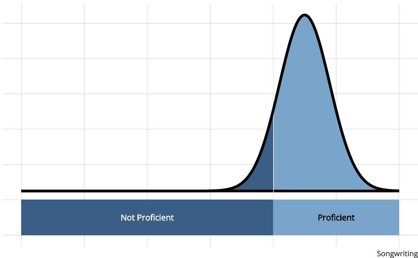
• Attributes are categorical, often dichotomous (e.g., proficient vs. non-proficient)

Diagnostic classification models

• DCMs place individuals into groups according to proficiency of multiple attributes

	songwriting	production	vocals	cohesion

Answering more questions

• Why is Taylor Swift (debut) so low?
  • Subpar songwriting, production, and vocals
• What aspects are albums competent/proficient in?
  • DCMs provide classifications directly

Diagnostic psychometrics

• Designed to be multidimensional
• No continuum of student achievement
• Categorical constructs
  • Usually binary (e.g., master/nonmaster, proficient/not proficient)
• Several different names in the literature
  • Diagnostic classification models (DCMs)
  • Cognitive diagnostic models (CDMs)
  • Skills assessment models
  • Latent response models
  • Restricted latent class models

Benefits of DCMs

• Fine-grained, multidimensional results
• Incorporates complex item structures
• High reliability with fewer items

Results from DCM-based assessments

	songwriting	production	vocals	cohesion

• No scale, no overall “ability”
• Students are probabilistically placed into classes
  • Classes are represented by skill profiles
• Feedback on specific skills as defined by the cognitive theory and test design

Item structures for DCMs

• Item structure: Which skills are measured by each item?

  • Simple structure: Item measures a single skill
  • Complex structure: Item measures 2+ skills

• Defined by Q-matrix

• Interactions between attributes when an item measures multiple skills driven by cognitive theory and/or empirical evidence

  • Can proficiency of one skill compensate for non-proficiency of another?
  • Are skill acquired in a particular order (e.g., hierarchy)?

item	songwriting	production	vocals	cohesion
1	1	1	0	0
2	1	0	0	0
3	1	0	0	1
4	0	0	0	1
5	1	0	1	0
6	0	1	0	1
7	1	0	0	0
8	1	0	1	0
9	0	0	1	0
10	0	1	1	0
11	1	0	1	0
12	0	0	0	1
13	0	0	1	0
14	1	0	0	0
15	0	1	0	0
16	1	1	0	0
17	0	0	1	1
18	0	0	0	1
19	0	1	0	0
20	0	0	1	1
21	0	1	0	0
22	1	0	0	0
23	0	0	0	1
24	0	0	1	0
25	0	0	1	1
26	0	1	1	0
27	0	0	1	0
28	1	1	0	0

Classification reliability

• Easier to categorize than place along a continuum

• Can set a proficiency threshold to optimize Type 1 or Type 2 errors

When are DCMs appropriate?

Success depends on:

1. Domain definitions
   • What are the attributes we’re trying to measure?
   • Are the attributes measurable (e.g., with assessment items)?
2. Alignment of purpose between assessment and model
   • Is classification the purpose?

Example applications

• Educational measurement: The competencies that student is or is not proficient in
  • Latent knowledge, skills, or understandings
  • Used for tailored instruction and remediation
• Psychiatric assessment: The DSM criteria that an individual meets
  • Broader diagnosis of a disorder

When are DCMs not appropriate?

• When the goal is to place individuals on a scale

• DCMs do not distinguish within classes

	songwriting	production	vocals	cohesion

Conceptual foundation summary

• DCMs are psychometric models designed to classify
  • We can define our attributes in any way that we choose
  • Items depend on the attribute definitions
  • Classifications are probabilistic
  • Takes fewer items to classify than to rank/scale

• DCMs provide valuable information with more feasible data demands than other psychometric models
  • Higher reliability than IRT/MIRT models
  • Naturally accommodates multidimensionality
  • Complex item structures possible
  • Criterion-referenced interpretations
  • Alignment of assessment goals and psychometric model

Statistical foundations

DCMs as statistical models

• Latent class models use responses to probabilistically place individuals into latent classes

• DCMs are confirmatory latent class models

  • Latent classes specified a priori as attribute profiles
  • Q-matrx specifies item-attribute structure
  • Person parameters are attribute proficiency probabilities

Terminology

• Respondents (r): The individuals from whom behavioral data are collected

  • For today, this is dichotomous assessment item responses
  • Not limited to only item responses in practice

• Items (i): Assessment questions used to classify/diagnose respondents

• Attributes (a): Unobserved latent categorical characteristics underlying the behaviors (i.e., diagnostic status)

  • Latent variables

• Diagnostic Assessment: The method used to elicit behavioral data

Attribute profiles

• With binary attributes, there are \(2^A\) possible profiles

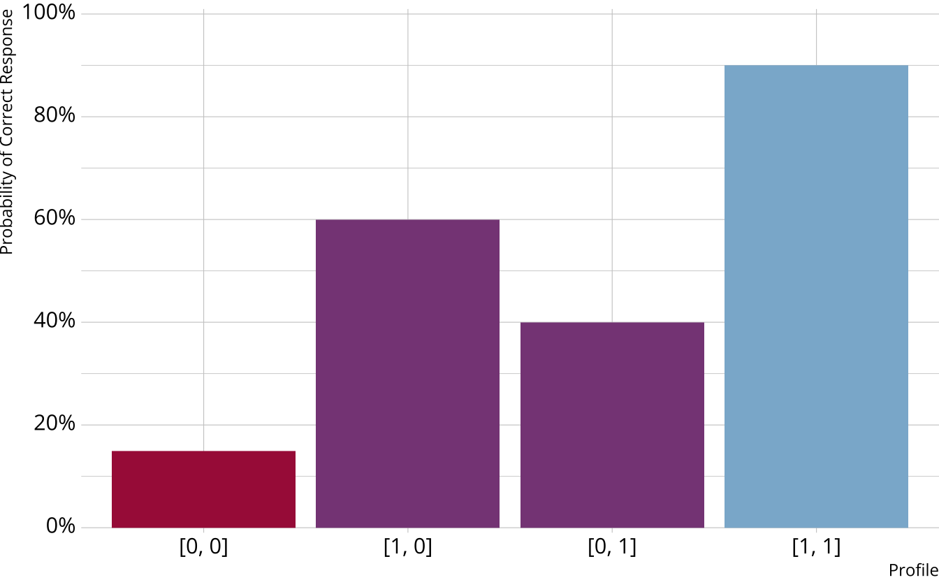
• Example 2-attribute assessment:

[0, 0]
[1, 0]
[0, 1]
[1, 1]

DCMs as latent class models

\[ \color{#D55E00}{P(X_r=x_r)} = \sum_{c=1}^C\color{#009E73}{\nu_c} \prod_{i=1}^I\color{#56B4E9}{\pi_{ic}^{x_{ir}}(1-\pi_{ic})^{1 - x_{ir}}} \]

Observed data: Probability of observing examinee r's item reponses

Structural component: Proportion of examinees in each class

Measurement component: Product of item response probabilities

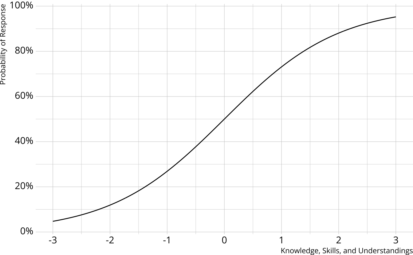
Measurement models

• Traditional psychometrics: Item response theory, classical test theory
  • A single, unidimensional construct
  • Student results estimated on a continuum
  • Performance on individual items determined by an “item characteristic curve”

Diagnostic assessment items

• Can be multidimensional

• No continuum of student achievement

• Categorical constructs

  • Usually binary (e.g., master/nonmaster, proficient/not proficient)

DCM measurement models

Reminder: We’re currently focusing on the measurement model.

\[ \color{#D55E00}{P(X_r=x_r)} = \sum_{c=1}^C\color{#009E73}{\nu_c} \prod_{i=1}^I\color{#56B4E9}{\pi_{ic}^{x_{ir}}(1-\pi_{ic})^{1 - x_{ir}}} \]

Different DCMs define π_ic in different ways

DCM measurement models

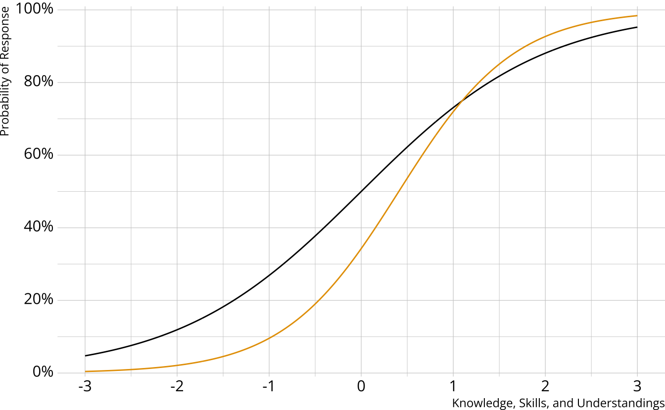
• Consider an assessment that measures 2 attributes

• With binary attributes there are \(2^A\) possible profiles

[0, 0]
[1, 0]
[0, 1]
[1, 1]

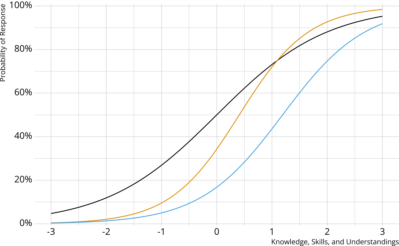
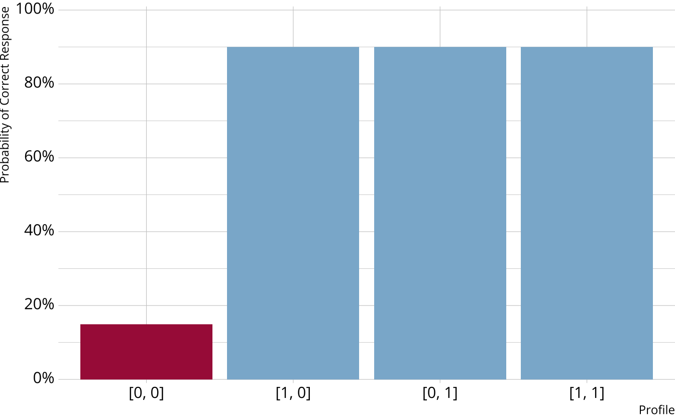
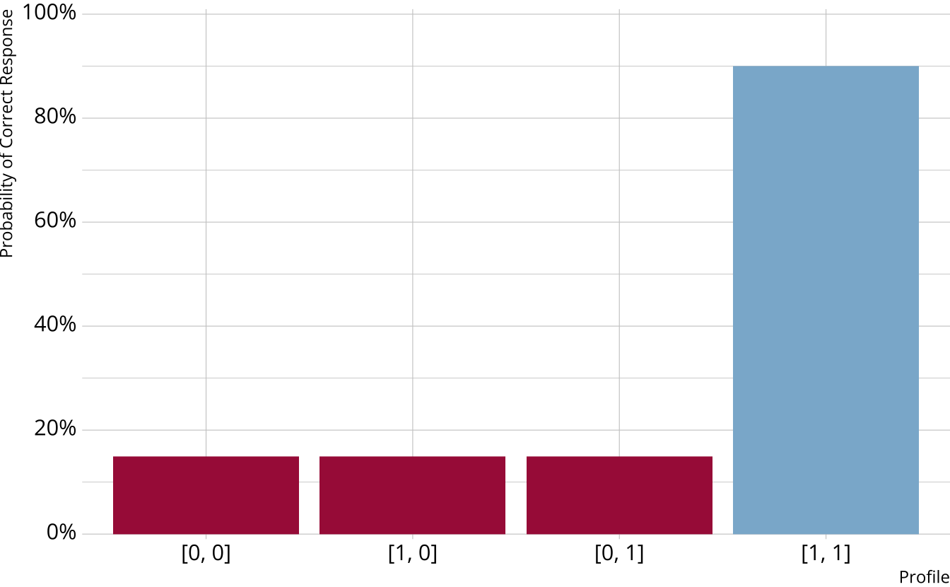
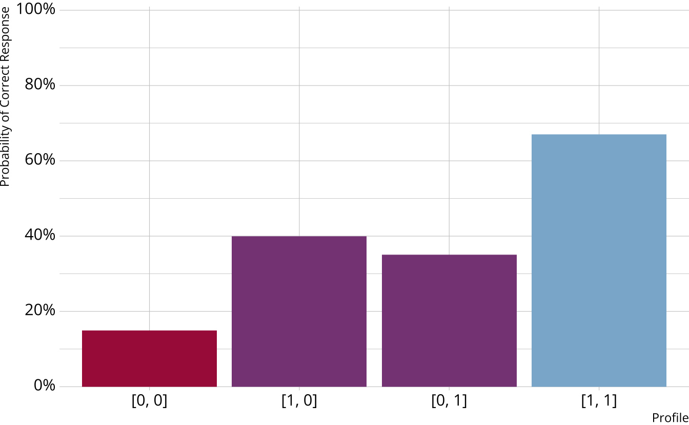
• Items can measure one or both attributes

• Item characteristic bar charts

Single-attribute DCM item

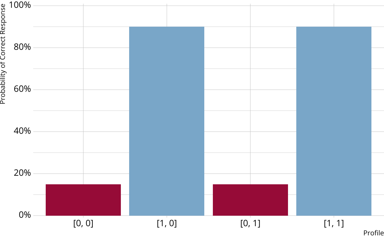
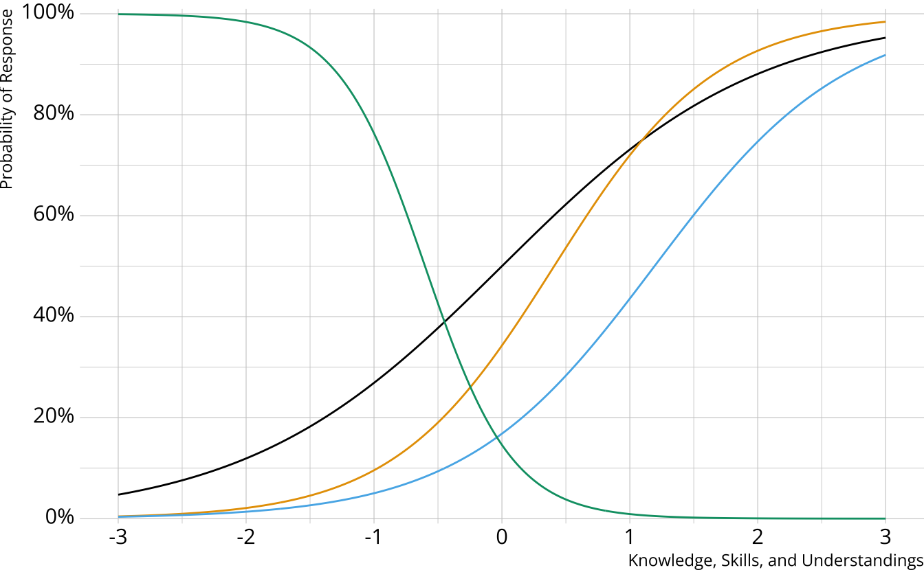
Multi-attribute items

• When items measure multiple attributes, what level of mastery is needed in order to provide a correct response?

• Many different types of DCMs that define this probability differently

  • Compensatory (e.g., DINO)
  • Noncompensatory (e.g., DINA)
  • Partially compensatory (e.g., C-RUM)

• General diagnostic models (e.g., LCDM)

• Each DCM makes different assumptions about how attributes proficiencies combine/interact to produce an item response

Compensatory DCMs

• Must be proficient in at least 1 attribute measured by the item to provide a correct response

• Deterministic inputs, noisy “or” gate (DINO; Templin & Henson, 2006)

Non-compensatory DCMs

• Must be proficient in all attributes measured by the item to provide a correct response

• Deterministic inputs, noisy “and” gate (DINA; de la Torre & Douglas, 2004)

Partially Compensatory DCMs

• Separate increases for each acquired attribute

• Compensatory reparameterized unified model (C-RUM; Hartz, 2002)

Which DCM to use?

• DINO, DINA, and C-RUM are just 3 of the MANY models that are available

• Each model comes with its own set of restrictions, and we typically have to specify a single model that is used for all items (software constraint)

• General form diagnostic models

  • Flexible; can subsume other more restrictive models
  • Again, several possibilities (e.g., G-DINA, GDM)
  • Loglinear cognitive diagnostic model

Loglinear cognitive diagnostic model (LCDM)

• Different response probabilities for each class (partially compensatory)

• Log-linear cognitive diagnostic model (LCDM; Henson et al., 2009)

Simple structure LCDM

Item measures only 1 attribute

\[ \text{logit}(X_i = 1) = \color{#A91E47}{\lambda_{i,0}} + \color{#8BB5D2}{\lambda_{i,1(1)}}\color{#81A757}{\alpha} \]

λ_i,0: Log-odds when not proficient

λ_i,1(1): Increase in log-odds when proficient

α: Attribute proficiency status (either 0 or 1)

Subscript notation

λ_i,e(α1)

• i = The item to which the parameter belongs

• e = The level of the effect
  • 0 = intercept
  • 1 = main effect
  • 2 = two-way interaction
  • 3 = three-way interaction
  • Etc.

• (α₁,…) = The attributes to which the effect applies
  • The same number of attributes as listed in subscript 2

Complex structure LCDM

Item measures multiple attributes

\[ \text{logit}(X_i = 1) = \color{#A91E47}{\lambda_{i,0}} + \color{#874886}{\lambda_{i,1(1)}\alpha_1} + \color{#96689A}{\lambda_{i,1(2)}\alpha_2} + \color{#8BB5D2}{\lambda_{i,2(1,2)}\alpha_1\alpha_2} \]

Log-odds when proficient in neither attribute

Increase in log-odds when proficient in attribute 1

Increase in log-odds when proficient in attribute 2

Change in log-odds when proficient in both attributes

Defining DCM structures

• Attribute and item relationships are defined in the Q-matrix

• Q-matrix

  • I \(\times\) A matrix
  • 0 = Attribute is not measured by the item
  • 1 = Attribute is measured by the item

The LCDM as a general DCM

• So called “general” DCM because the LCDM subsumes other DCMs

• Constraints on item parameters make LCDM equivalent to other DCMs (e.g., DINA and DINO)

  • Interactive Shiny app: https://atlas-aai.shinyapps.io/dcm-probs/
  • DINA
    • Only the intercept and highest-order interaction are non-0
  • DINO
    • All main effects are equal
    • All two-way interactions are -1 \(\times\) main effect
    • All three-way interactions are -1 \(\times\) two-way interaction (i.e., equal to main effects)
    • Etc.
  • C-RUM
    • Only the intercept and main effects are non-0 (i.e., interactions are not estimated)

• Testable hypotheses!

Estimation and Evaluation

Model Estimation

What is measr?

• R package that provides a fully Bayesian estimation of DCMs using Stan
• Provides additional functions to automate the evaluation of DCMs
  • Model fit
  • Classification accuracy and consistency

Example data

• Read data
• Data
• Q-matrix

• Simulated data: https://bit.ly/sp24-epsy896-dcm

ts_dat <- read_rds(here("data", "taylor-data.rds"))
ts_qmat <- read_rds(here("data", "taylor-qmatrix.rds"))

ts_dat

# A tibble: 500 × 29
   album   `1`   `2`   `3`   `4`   `5`   `6`   `7`   `8`   `9`  `10`  `11`  `12`
   <chr> <int> <int> <int> <int> <int> <int> <int> <int> <int> <int> <int> <int>
 1 Melo…     0     1     1     1     0     1     0     0     1     1     0     0
 2 A Ni…     1     0     0     0     0     0     0     0     0     0     0     0
 3 Cann…     1     0     0     0     0     0     1     0     0     0     0     0
 4 BORN…     1     0     0     1     1     0     0     0     1     0     0     0
 5 Loose     1     0     0     1     1     1     0     0     0     1     1     1
 6 Red       0     1     0     0     1     1     0     1     0     0     1     0
 7 Wild…     0     0     1     1     0     0     0     0     1     0     0     1
 8 Dawn…     0     0     1     1     0     1     0     1     0     0     0     0
 9 than…     0     0     0     0     0     0     0     0     1     1     0     1
10 In A…     1     0     1     1     0     1     1     0     0     0     0     0
# ℹ 490 more rows
# ℹ 16 more variables: `13` <int>, `14` <int>, `15` <int>, `16` <int>,
#   `17` <int>, `18` <int>, `19` <int>, `20` <int>, `21` <int>, `22` <int>,
#   `23` <int>, `24` <int>, `25` <int>, `26` <int>, `27` <int>, `28` <int>

ts_qmat

# A tibble: 28 × 4
   songwriting production vocals cohesion
         <int>      <int>  <int>    <int>
 1           1          1      0        0
 2           1          0      0        0
 3           1          0      0        1
 4           0          0      0        1
 5           1          0      1        0
 6           0          1      0        1
 7           1          0      0        0
 8           1          0      1        0
 9           0          0      1        0
10           0          1      1        0
# ℹ 18 more rows

measr_dcm()

Estimate a DCM with Stan

ts_dcm <- measr_dcm(
1  data = ts_dat, qmatrix = ts_qmat,
  resp_id = "album",
2  type = "lcdm",
3  method = "mcmc", backend = "cmdstanr",
4  iter_warmup = 1500, iter_sampling = 500,
  chains = 4, parallel_chains = 4,
5  file = "fits/taylor-lcdm"
)

1

Specify your data, Q-matrix, and ID columns

2

Choose the DCM to estimate (e.g., LCDM, DINA, etc.)

3

Choose the estimation engine

4

Pass additional arguments to rstan or cmdstanr

5

Save the model to save time in the future

measr_dcm() options

• type: Declare the type of DCM to estimate. Currently supports LCDM, DINA, DINO, and C-RUM

• method: How to estimate the model. To sample, use “mcmc”. To use Stan’s optimizer, use “optim”

• backend: Which engine to use, either “rstan” or “cmdstanr”

• ...: Additional arguments that are passed to, depending on the method and backend:

  • rstan::sampling()
  • rstan::optimizing()
  • cmdstanr::sample()
  • cmdstanr::optimize()

View predictions

• Calcualte results
• Class-level
• Attribute-level
• Taylor Results

• Two types of results
  • Class-level results
  • Attribute-level results

ts_results <- predict(ts_dcm, summary = FALSE)

ts_results$class_probabilities

# A tibble: 500 × 17
   album                       `[0,0,0,0]`        `[1,0,0,0]`        `[0,1,0,0]`
   <fct>                        <rvar[1d]>         <rvar[1d]>         <rvar[1d]>
 1 Melodrama             1.1e-06 ± 1.2e-06  1.3e-08 ± 1.4e-08  3.7e-05 ± 3.0e-05
 2 A Night At The Oper…  9.5e-01 ± 2.3e-02  8.5e-03 ± 5.1e-03  8.5e-03 ± 5.3e-03
 3 Cannibal (Expanded …  1.2e-02 ± 9.4e-03  4.2e-03 ± 3.4e-03  9.1e-01 ± 4.7e-02
 4 BORN PINK             1.5e-01 ± 7.1e-02  1.6e-04 ± 1.2e-04  3.1e-01 ± 1.2e-01
 5 Loose                 8.5e-06 ± 9.6e-06  5.1e-08 ± 6.1e-08  1.5e-04 ± 1.2e-04
 6 Red                   1.8e-03 ± 1.9e-03  1.4e-02 ± 1.2e-02  9.7e-02 ± 6.2e-02
 7 Wildfire              1.7e-04 ± 1.5e-04  1.6e-07 ± 1.7e-07  1.4e-03 ± 1.3e-03
 8 Dawn FM               5.4e-05 ± 6.1e-05  2.6e-07 ± 2.8e-07  1.2e-03 ± 7.5e-04
 9 thank u, next         7.1e-02 ± 4.9e-02  5.8e-06 ± 4.9e-06  3.7e-02 ± 2.5e-02
10 In A Perfect World …  1.2e-08 ± 1.6e-08  7.1e-05 ± 5.7e-05  9.8e-07 ± 8.7e-07
# ℹ 490 more rows
# ℹ 13 more variables: `[0,0,1,0]` <rvar[1d]>, `[0,0,0,1]` <rvar[1d]>,
#   `[1,1,0,0]` <rvar[1d]>, `[1,0,1,0]` <rvar[1d]>, `[1,0,0,1]` <rvar[1d]>,
#   `[0,1,1,0]` <rvar[1d]>, `[0,1,0,1]` <rvar[1d]>, `[0,0,1,1]` <rvar[1d]>,
#   `[1,1,1,0]` <rvar[1d]>, `[1,1,0,1]` <rvar[1d]>, `[1,0,1,1]` <rvar[1d]>,
#   `[0,1,1,1]` <rvar[1d]>, `[1,1,1,1]` <rvar[1d]>

ts_results$attribute_probabilities

# A tibble: 500 × 5
   album                       songwriting       production               vocals
   <fct>                        <rvar[1d]>       <rvar[1d]>           <rvar[1d]>
 1 Melodrama           0.000419 ± 0.000278  0.9422 ± 0.0340  0.966461 ± 0.019196
 2 A Night At The Op…  0.008565 ± 0.005107  0.0086 ± 0.0053  0.033112 ± 0.019671
 3 Cannibal (Expande…  0.080788 ± 0.044734  0.9842 ± 0.0114  0.000045 ± 0.000039
 4 BORN PINK           0.000471 ± 0.000233  0.3845 ± 0.1307  0.508834 ± 0.137168
 5 Loose               0.001590 ± 0.001057  0.8967 ± 0.0614  0.935788 ± 0.042500
 6 Red                 0.746107 ± 0.099693  0.6544 ± 0.1407  0.703408 ± 0.128450
 7 Wildfire            0.000059 ± 0.000035  0.1359 ± 0.1027  0.951212 ± 0.028540
 8 Dawn FM             0.000650 ± 0.000407  0.9544 ± 0.0313  0.003481 ± 0.003005
 9 thank u, next       0.000020 ± 0.000010  0.2147 ± 0.0833  0.890630 ± 0.065815
10 In A Perfect Worl…  0.997949 ± 0.001355  0.9638 ± 0.0216  0.004456 ± 0.004106
# ℹ 490 more rows
# ℹ 1 more variable: cohesion <rvar[1d]>

ts_results$attribute_probabilities |> 
  semi_join(taylor_albums, join_by(album == album_name))

# A tibble: 14 × 5
   album                        songwriting        production             vocals
   <fct>                         <rvar[1d]>        <rvar[1d]>         <rvar[1d]>
 1 Red                  0.746107 ± 0.099693  0.6544 ± 0.14069  0.70341 ± 0.12845
 2 Fearless (Taylor's…  0.915897 ± 0.058410  0.0308 ± 0.02352  0.02697 ± 0.01902
 3 Speak Now (Taylor'…  0.999783 ± 0.000145  0.2619 ± 0.12795  0.12060 ± 0.07406
 4 Midnights            0.997510 ± 0.001928  0.0206 ± 0.01822  0.86307 ± 0.09284
 5 reputation           0.561946 ± 0.157150  0.0631 ± 0.04698  0.95791 ± 0.02410
 6 Red (Taylor's Vers…  0.999976 ± 0.000017  0.9808 ± 0.01220  0.97884 ± 0.01149
 7 Fearless             0.527831 ± 0.173573  0.0092 ± 0.00751  0.00091 ± 0.00068
 8 1989 (Taylor's Ver…  0.195956 ± 0.116831  0.9960 ± 0.00250  0.99601 ± 0.00216
 9 Taylor Swift         0.000055 ± 0.000031  0.0012 ± 0.00073  0.00011 ± 0.00008
10 folklore             0.999904 ± 0.000074  0.9855 ± 0.01114  0.99407 ± 0.00352
11 Speak Now            0.575813 ± 0.147118  0.3276 ± 0.13558  0.00072 ± 0.00052
12 evermore             0.826752 ± 0.077166  0.9304 ± 0.04031  0.91412 ± 0.04216
13 Lover                0.494974 ± 0.152578  0.0016 ± 0.00140  0.89823 ± 0.06781
14 1989                 0.000043 ± 0.000025  0.9465 ± 0.03016  0.84713 ± 0.07194
# ℹ 1 more variable: cohesion <rvar[1d]>

Model Evaluation

How to evaluate DCMs?

• Three types of model evaluation we’ll discuss:
  • Absolute model fit
  • Relative model fit
  • Reliability

Absolute fit

• How well does the model fit the data?

• Overall model fit

  • M₂ (Liu et al., 2016)
  • Posterior predictive model checks (PPMCs; Thompson, 2019)

• Item-level fit

  • PPMCs (Sinharay & Almond, 2007)

M₂

• For the M₂ statistic, p-values greater than .05 indicate acceptable fit

fit_m2(ts_dcm)

# A tibble: 1 × 8
     m2    df  pval   rmsea ci_lower ci_upper `90% CI`     srmsr
  <dbl> <int> <dbl>   <dbl>    <dbl>    <dbl> <chr>        <dbl>
1  310.   309 0.478 0.00218        0   0.0173 [0, 0.0173] 0.0371

• The fit_m2() function also returns some other model fit statistics that may be familiar
  • RMSEA: root mean square error of approximation
  • SRMSR: standardized root mean square residual

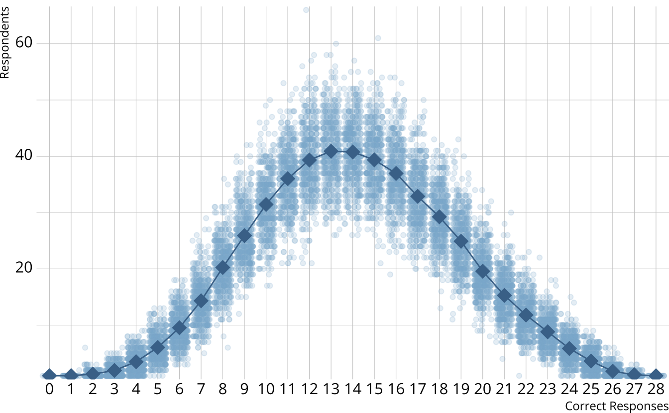
PPMC: Raw score distribution

• For each iteration, calculate the total number of respondents at each score point

• Calculate the expected number of respondents at each score point

• Calculate the observed number of respondents at each score point

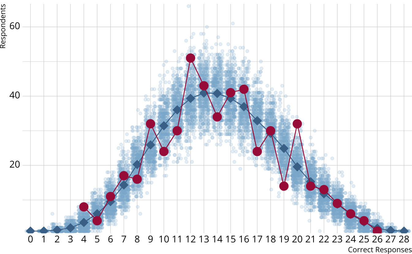
PPMC: \(\chi^2\)

• Calculate a \(\chi^2\)-like statistic comparing the number of respondents at each score point in each iteration to the expectation

• Calculate the \(\chi^2\) value comparing the observed data to the expectation

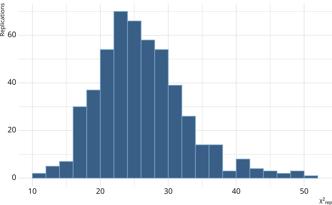
PPMC: ppp

• Calculate the proportion of iterations where the \(\chi^2\)-like statistic from replicated data set exceed the observed data statistic
  • Posterior predictive p-value (ppp)
  • ppp values between .025 and .975 represent acceptable model fit

fit_ppmc(ts_dcm, model_fit = "raw_score", item_fit = NULL)

# A tibble: 1 × 5
  obs_chisq ppmc_mean `2.5%` `97.5%`   ppp
      <dbl>     <dbl>  <dbl>   <dbl> <dbl>
1      35.9      30.7   14.9    57.1 0.207

PPMC: Item-level fit

• Item-level fit
• Conditional probabilities
• Odds ratios

• We can also use PPMCs to calculate item-level statistics
  • Conditional probabilities of classes providing a correct response
  • Odds ratios between item pairs

fit_ppmc(ts_dcm, model_fit = NULL, item_fit = "conditional_prob")

# A tibble: 448 × 7
   item  class     obs_cond_pval ppmc_mean `2.5%` `97.5%`    ppp
   <fct> <chr>             <dbl>     <dbl>  <dbl>   <dbl>  <dbl>
 1 1     [0,0,0,0]         0.162     0.207  0.135   0.274 0.894 
 2 1     [1,0,0,0]         0.609     0.629  0.537   0.714 0.668 
 3 1     [0,1,0,0]         0.429     0.320  0.243   0.409 0.01  
 4 1     [0,0,1,0]         0.332     0.207  0.135   0.274 0.0005
 5 1     [0,0,0,1]         0.166     0.207  0.135   0.274 0.866 
 6 1     [1,1,0,0]         0.628     0.733  0.645   0.821 0.992 
 7 1     [1,0,1,0]         0.759     0.629  0.537   0.714 0.0005
 8 1     [1,0,0,1]         0.522     0.629  0.537   0.714 0.988 
 9 1     [0,1,1,0]         0.277     0.320  0.243   0.409 0.847 
10 1     [0,1,0,1]         0.298     0.320  0.243   0.409 0.679 
# ℹ 438 more rows

fit_ppmc(ts_dcm, model_fit = NULL, item_fit = "odds_ratio")

# A tibble: 378 × 7
   item_1 item_2 obs_or ppmc_mean `2.5%` `97.5%`   ppp
   <fct>  <fct>   <dbl>     <dbl>  <dbl>   <dbl> <dbl>
 1 1      2       2.13       2.65  1.67     4.02 0.818
 2 1      3       1.51       1.94  1.27     2.86 0.868
 3 1      4       0.906      1.13  0.760    1.62 0.846
 4 1      5       1.78       1.53  0.986    2.21 0.190
 5 1      6       1.35       1.27  0.846    1.84 0.34 
 6 1      7       4.17       3.36  2.02     5.40 0.16 
 7 1      8       2.02       1.98  1.30     2.93 0.413
 8 1      9       0.939      1.04  0.717    1.48 0.664
 9 1      10      1.17       1.12  0.740    1.60 0.368
10 1      11      1.82       1.75  1.12     2.60 0.373
# ℹ 368 more rows

Relative fit

• Doesn’t give us information whether or not a model fits the data, only compares competing models to each other
  • Should be evaluated in conjunction with absolute model fit
• Several options available for Bayesian models
  • PSIS-LOO (Vehtari, 2017)
  • WAIC (Watanabe, 2010)

Comparison model

• For a comparison, let’s estimate a DINA model to our same data set
  • Reminder: DINA is a more restrictive model than the LCDM

ts_dina <- measr_dcm(
  data = ts_dat, qmatrix = ts_qmat,
  resp_id = "album",
  type = "dina",
  method = "mcmc", backend = "cmdstanr",
  iter_warmup = 1500, iter_sampling = 500,
  chains = 4, parallel_chains = 4,
  file = "fits/taylor-dina"
)

Model comparison

• Comparisons
• LOO
• WAIC

• Calculate information criteria with loo() or waic()
• Compare using loo_compare()
• If the absolute value of the difference is greater than 2.5 × standard error, that indicates a preference for the model in the first row

lcdm_loo <- loo(ts_dcm)
dina_loo <- loo(ts_dina)

loo_compare(list(lcdm = lcdm_loo, dina = dina_loo))

     elpd_diff se_diff
lcdm    0.0       0.0 
dina -377.7      19.2 

lcdm_waic <- waic(ts_dcm)
dina_waic <- waic(ts_dina)

loo_compare(list(lcdm = lcdm_waic, dina = dina_waic))

     elpd_diff se_diff
lcdm    0.0       0.0 
dina -394.9      19.9 

Reliability

• Reporting reliability depends on how results are estimated and reported

• Reliability for:

  • Profile-level classification
  • Attribute-level classification
  • Attribute-level probability of proficiency

ts_reli <- reliability(ts_dcm)

Profile-level classification

• Profile-level probabilities
• Profile-level classifications
• Profile reliability

ts_results$class_probabilities

# A tibble: 500 × 17
   album                       `[0,0,0,0]`        `[1,0,0,0]`        `[0,1,0,0]`
   <fct>                        <rvar[1d]>         <rvar[1d]>         <rvar[1d]>
 1 Melodrama             1.1e-06 ± 1.2e-06  1.3e-08 ± 1.4e-08  3.7e-05 ± 3.0e-05
 2 A Night At The Oper…  9.5e-01 ± 2.3e-02  8.5e-03 ± 5.1e-03  8.5e-03 ± 5.3e-03
 3 Cannibal (Expanded …  1.2e-02 ± 9.4e-03  4.2e-03 ± 3.4e-03  9.1e-01 ± 4.7e-02
 4 BORN PINK             1.5e-01 ± 7.1e-02  1.6e-04 ± 1.2e-04  3.1e-01 ± 1.2e-01
 5 Loose                 8.5e-06 ± 9.6e-06  5.1e-08 ± 6.1e-08  1.5e-04 ± 1.2e-04
 6 Red                   1.8e-03 ± 1.9e-03  1.4e-02 ± 1.2e-02  9.7e-02 ± 6.2e-02
 7 Wildfire              1.7e-04 ± 1.5e-04  1.6e-07 ± 1.7e-07  1.4e-03 ± 1.3e-03
 8 Dawn FM               5.4e-05 ± 6.1e-05  2.6e-07 ± 2.8e-07  1.2e-03 ± 7.5e-04
 9 thank u, next         7.1e-02 ± 4.9e-02  5.8e-06 ± 4.9e-06  3.7e-02 ± 2.5e-02
10 In A Perfect World …  1.2e-08 ± 1.6e-08  7.1e-05 ± 5.7e-05  9.8e-07 ± 8.7e-07
# ℹ 490 more rows
# ℹ 13 more variables: `[0,0,1,0]` <rvar[1d]>, `[0,0,0,1]` <rvar[1d]>,
#   `[1,1,0,0]` <rvar[1d]>, `[1,0,1,0]` <rvar[1d]>, `[1,0,0,1]` <rvar[1d]>,
#   `[0,1,1,0]` <rvar[1d]>, `[0,1,0,1]` <rvar[1d]>, `[0,0,1,1]` <rvar[1d]>,
#   `[1,1,1,0]` <rvar[1d]>, `[1,1,0,1]` <rvar[1d]>, `[1,0,1,1]` <rvar[1d]>,
#   `[0,1,1,1]` <rvar[1d]>, `[1,1,1,1]` <rvar[1d]>

# A tibble: 14 × 3
   album                        profile    prob
   <fct>                        <chr>     <dbl>
 1 Red                          [1,0,1,0] 0.297
 2 Fearless (Taylor's Version)  [1,0,0,1] 0.869
 3 Speak Now (Taylor's Version) [1,0,0,0] 0.351
 4 Midnights                    [1,0,1,1] 0.831
 5 reputation                   [1,0,1,0] 0.517
 6 Red (Taylor's Version)       [1,1,1,0] 0.488
 7 Fearless                     [1,0,0,1] 0.523
 8 1989 (Taylor's Version)      [0,1,1,1] 0.797
 9 Taylor Swift                 [0,0,0,1] 0.878
10 folklore                     [1,1,1,1] 0.979
11 Speak Now                    [1,0,0,0] 0.479
12 evermore                     [1,1,1,1] 0.704
13 Lover                        [0,0,1,1] 0.442
14 1989                         [0,1,1,1] 0.797

ts_reli$pattern_reliability

      p_a       p_c 
0.7819620 0.6279945 

• Estimating classification consistency and accuracy for cognitive diagnostic assessment (Cui et al., 2012)

Attribute-level classification

• Attribute-level probabilities
• Attribute-level classifications
• Classification reliability

ts_results$attribute_probabilities

# A tibble: 500 × 5
   album                       songwriting       production               vocals
   <fct>                        <rvar[1d]>       <rvar[1d]>           <rvar[1d]>
 1 Melodrama           0.000419 ± 0.000278  0.9422 ± 0.0340  0.966461 ± 0.019196
 2 A Night At The Op…  0.008565 ± 0.005107  0.0086 ± 0.0053  0.033112 ± 0.019671
 3 Cannibal (Expande…  0.080788 ± 0.044734  0.9842 ± 0.0114  0.000045 ± 0.000039
 4 BORN PINK           0.000471 ± 0.000233  0.3845 ± 0.1307  0.508834 ± 0.137168
 5 Loose               0.001590 ± 0.001057  0.8967 ± 0.0614  0.935788 ± 0.042500
 6 Red                 0.746107 ± 0.099693  0.6544 ± 0.1407  0.703408 ± 0.128450
 7 Wildfire            0.000059 ± 0.000035  0.1359 ± 0.1027  0.951212 ± 0.028540
 8 Dawn FM             0.000650 ± 0.000407  0.9544 ± 0.0313  0.003481 ± 0.003005
 9 thank u, next       0.000020 ± 0.000010  0.2147 ± 0.0833  0.890630 ± 0.065815
10 In A Perfect Worl…  0.997949 ± 0.001355  0.9638 ± 0.0216  0.004456 ± 0.004106
# ℹ 490 more rows
# ℹ 1 more variable: cohesion <rvar[1d]>

# A tibble: 14 × 5
   album                        songwriting production vocals cohesion
   <fct>                              <int>      <int>  <int>    <int>
 1 Red                                    1          1      1        0
 2 Fearless (Taylor's Version)            1          0      0        1
 3 Speak Now (Taylor's Version)           1          0      0        0
 4 Midnights                              1          0      1        1
 5 reputation                             1          0      1        0
 6 Red (Taylor's Version)                 1          1      1        0
 7 Fearless                               1          0      0        1
 8 1989 (Taylor's Version)                0          1      1        1
 9 Taylor Swift                           0          0      0        1
10 folklore                               1          1      1        1
11 Speak Now                              1          0      0        0
12 evermore                               1          1      1        1
13 Lover                                  0          0      1        1
14 1989                                   0          1      1        1

ts_reli$map_reliability

$accuracy
# A tibble: 4 × 8
  attribute     acc lambda_a kappa_a youden_a tetra_a  tp_a  tn_a
  <chr>       <dbl>    <dbl>   <dbl>    <dbl>   <dbl> <dbl> <dbl>
1 songwriting 0.973    0.944   0.399    0.946   0.996 0.971 0.975
2 production  0.900    0.800   0.784    0.800   0.951 0.901 0.899
3 vocals      0.927    0.848   0.849    0.855   0.974 0.933 0.922
4 cohesion    0.958    0.916   0.413    0.917   0.992 0.961 0.956

$consistency
# A tibble: 4 × 10
  attribute   consist lambda_c kappa_c youden_c tetra_c  tp_c  tn_c gammak
  <chr>         <dbl>    <dbl>   <dbl>    <dbl>   <dbl> <dbl> <dbl>  <dbl>
1 songwriting   0.949    0.895   0.944    0.898   0.987 0.947 0.951  0.958
2 production    0.823    0.644   0.800    0.646   0.849 0.824 0.822  0.855
3 vocals        0.865    0.724   0.853    0.730   0.912 0.862 0.868  0.891
4 cohesion      0.920    0.838   0.916    0.841   0.969 0.922 0.919  0.940
# ℹ 1 more variable: pc_prime <dbl>

• Measures of agreement to assess attribute-level classification accuracy and consistency for cognitive diagnostic assessments (Johnson & Sinharay, 2018)

Attribute-level probabilities

• Attribute-level probabilities
• Probability reliability

ts_results$attribute_probabilities

# A tibble: 500 × 5
   album                       songwriting       production               vocals
   <fct>                        <rvar[1d]>       <rvar[1d]>           <rvar[1d]>
 1 Melodrama           0.000419 ± 0.000278  0.9422 ± 0.0340  0.966461 ± 0.019196
 2 A Night At The Op…  0.008565 ± 0.005107  0.0086 ± 0.0053  0.033112 ± 0.019671
 3 Cannibal (Expande…  0.080788 ± 0.044734  0.9842 ± 0.0114  0.000045 ± 0.000039
 4 BORN PINK           0.000471 ± 0.000233  0.3845 ± 0.1307  0.508834 ± 0.137168
 5 Loose               0.001590 ± 0.001057  0.8967 ± 0.0614  0.935788 ± 0.042500
 6 Red                 0.746107 ± 0.099693  0.6544 ± 0.1407  0.703408 ± 0.128450
 7 Wildfire            0.000059 ± 0.000035  0.1359 ± 0.1027  0.951212 ± 0.028540
 8 Dawn FM             0.000650 ± 0.000407  0.9544 ± 0.0313  0.003481 ± 0.003005
 9 thank u, next       0.000020 ± 0.000010  0.2147 ± 0.0833  0.890630 ± 0.065815
10 In A Perfect Worl…  0.997949 ± 0.001355  0.9638 ± 0.0216  0.004456 ± 0.004106
# ℹ 490 more rows
# ℹ 1 more variable: cohesion <rvar[1d]>

ts_reli$eap_reliability

# A tibble: 4 × 5
  attribute   rho_pf rho_bs rho_i rho_tb
  <chr>        <dbl>  <dbl> <dbl>  <dbl>
1 songwriting  0.920  0.917 0.710  0.991
2 production   0.715  0.710 0.595  0.898
3 vocals       0.783  0.782 0.637  0.942
4 cohesion     0.880  0.880 0.692  0.982

• The reliability of the posterior probability of skill attainment in diagnostic classification models (Johnson & Sinharay, 2020)

Summary

Diagnostic classification models

• Confirmatory latent class models with categorical latent variables

• Many benefits over traditional methods

  • Fine-grained, multidimensional results
  • Incorporates complex item structures
  • High reliability with fewer items

• Broad applicability in educational and psychological measurement

Learn more about DCMs

Learn more about measr

measr documentation

wjakethompson/measr

https://epsy896-dcm.wjakethompson.com

wjakethompson.com
wjakethompson@ku.edu
@wjakethompson
@wjakethompson.com
@wjakethompson@fosstodon.org
@wjakethompson